
Read this Before Creating Your Next Index in PSQL
My friends used to poke me for writing long messages while texting. I thought why not benefit from it? I have led communities, ran startups, built viral apps, and made youtube vlogs.. Yes, I am an engineer.
If you are a beginner in your developer journey tasked with optimizing a database query, you must have read about applying indexes. But not all indexes bring performance gains. Some can even degrade it. Read this blog before your create your next index.

How Indexing Works in PSQL
Query Planner
Whenever you run a query on your database, a query planner analyzes the query and creates a plan to execute it. This plan optimizes for performance. It focuses on the following aspects: the number of workers to use, scan strategy (sequential or indexed), and whether to use in-memory or file storage sorting. It also estimates the time to execute and records (tuples) that will be fetched during the query. All this is estimated by analyzing historical data trends (PG statistics). By adding “explain” before your query, you can access the above-mentioned query plan.
EXPLAIN ANALYZE
SELECT count(*) FROM invoices
WHERE billing_country = 'india';
Query Response:
| Aggregate (cost=10000000012.38..10000000012.39 rows=1 width=8) (actual time=0.100..0.100 rows=1 loops=1) |
| -> Seq Scan on invoices (cost=10000000000.00..10000000012.38 rows=1 width=0) (actual time=0.100..0.100 rows=0 loops=1) |
| Filter: ((billing_country)::text = 'india'::text) |
| Rows Removed by Filter: 10 |
| Planning Time: 0.200 ms |
| Execution Time: 0.100 ms |
link for accessing the above mentioned playground database.
Before creating any index, you should read the query plan of the commonly used queries that will be affected by the index. Since this plan is based on historical data, it is important that your metrics are updated continuously. This is handled by running “vacuum analyze” on your table.
vacuum analyze invoices
Sequential Scan vs Indexed Scan
The cost of executing a query is directly proportional to the number of tuples or DB pages it fetches. Say the cost of fetching records by performing a sequential scan is X units. Then, for fetching 1 lakh pages, the cost will be 100k into X units. These records are fetched in a sequential manner, resulting in less cost for accessing continuous records.
Similarly, when utilizing an index, the cost of fetching a page from a table can be 4X units. This is more than the cost of accessing a page in a sequential scan. This is because your index stores tuple references. To access the data, the query executor needs to fetch pages from the actual disk storage. This access can be in a random manner. Therefore, the DB query engine adds a punishing cost for this random behavior. As a result, the cost per page can be up to 4 times the cost of accessing records in a sequential manner.

So, it all boils down to the number of records (database pages) fetched. If by using an index, the query planner estimates it will have to fetch about 40k records, the cost will be rough around 40,000 * 4 X = 160,000 units. This cost is higher than performing a sequential scan involving the fetching of 1 lakh records. Hence query planner may prefer not using the index. This is an important aspect in deciding if adding an index will help in your case or not.
There’s one important consideration. When using high speed storage hardware like SSD for your database physical storage, the penalty of accessing entries in a random order may not be 4 times the cost of accessing them sequentially. This parameter can then be tuned accordingly in such situations as per your specific needs.
Selectivity of Your Index
In the above section, we discussed how the total number of records to be fetched has a direct impact on your overall query performance. To promote the usage of your index, it is important for your query to return less number of records or be more selective. To identify this information, you can refer to the cost estimates in your query planner results. It shows the estimated number of records to be fetched.
Additionally, the query planner estimates the record count by reading values from the historical data we discussed above. PG statistics contain information about the data distribution of all your tables.
SELECT * FROM pg_stats
WHERE tablename = 'invoices'
Query Response:
| TABLENAME | ATTNAME | MOST_COMMON_VALS | MOST_COMMON_FREQS | CORRELATION | HISTOGRAM_BOUNDS |
| invoices | billing_address | NULL | NULL | NULL | NULL |
| invoices | invoice_id | NULL | NULL | 1 | {1,2,3,4,5,6,7,8,9,10} |
| invoices | customer_id | {1,2,3,4,5} | 0.2,0.2,0.2,0.2,0.2 | 0.6364 | NULL |
| invoices | invoice_date | NULL | NULL | 1 | {"2021-01-01 00:00:00","2021-01-02 00:00:00","2021-01-03 00:00:00","2021-01-06 00:00:00","2021-01-11 00:00:00","2021-02-01 00:00:00","2021-02-02 00:00:00","2021-02-08 00:00:00","2021-02-11 00:00:00","2021-02-19 00:00:00"} |
| invoices | billing_city | {Montreal,Oslo,Prague,"Sao Paulo",Stuttgart} | 0.2,0.2,0.2,0.2,0.2 | -0.0909 | NULL |
| invoices | billing_country | {Brazil,Canada,"Czech Republic",Germany,Norway} | 0.2,0.2,0.2,0.2,0.2 | 0.3939 | NULL |
| invoices | total | {1.98,3.96,5.94} | 0.3,0.2,0.2 | 0.1152 | {0.99,8.91,13.86} |
Here is a brief explanation about some of the fields shown above:
Most_common_vals - some of the values that appear frequently in a column.
Most_common_freqs - for each of the frequently occurring values, this shows their frequency in percentage [in decimals]. So to estimate how many records exist with a value of billing country as Brazil, we can multiply the total number of records in the table by the frequency of Brazil, i.e., 0.2
Correlation - it describes how correlated the values are with each other. A correlation value nearing 1 or -1 demonstrates a strong correlation. This reduces random access cost when fetching records in a range. (more on this later)
Histogram_bounds - for range-based queries (date > yesterday), the estimated records are fetched by multiplying the records in each histogram interval.
I have used the above command numerous times to identify the distinct values and their frequencies. If you are querying on a single column with very low distinct values, or on a value that appears very frequently (high most_common_freq), chances are the query planner will always favor a sequential scan over an index scan in a table with a large number of records.
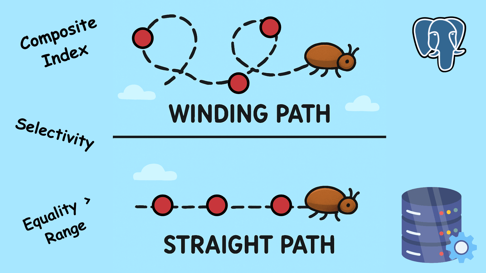
Composite Index
A composite index is made on two or more columns. Here ordering of the columns matters greatly. Say you have an index on columns A, B, and C. When querying over only A or A and B, your index is used. However, when querying over only C or A and C, there is a chance that this index is not used. This is because in an index, entries are stored by sorting them on value A, then value B, and then value C. So querying directly on value C via an index made on A, B, and C is not optimal in most cases. Hence, it is advised to order your columns in index as per your query pattern. While some people suggest ordering on the basis of selectivity (more selective values earlier), there’s one more advice that you should consider.
Equality Over Range
If your query is filtering on Col B with an equality symbol ( = ) and then on Column C using a range filter ( ≥= ), then more priority should be given to Col B in the ordering of the index. This is because, by having an index over B and C, your query planner will find the first possible record and then perform a sequential scan to satisfy the range filter. This reduces the number of tuples fetched in random order from the heap. Adding a reverse index will not allow this possibility to hold true. Hence, it is advised to value the relational signs in your query as well while deciding the ordering of columns in your index.
Index Only Scan
The query executor has to fetch tuples from the heap since the index generally stores a reference to your original tuple along with the data used to create the index. In case your query only needs the data stored in the index, it can result into an index only scan, removing the need to fetch records from the tuple. To fully utilize the performance gain from an index-only scan, you can store additional data in your index without creating an index on those columns. For e.g, if your table has 7 columns and your top query fetches data from 3 columns only. In case the query is only filtering on 1 column, you can create an index on that column and store the data for the additional two columns in that same index using the include command.
CREATE INDEX idx_billing_country ON invoices (billing_country) INCLUDE (payment_method)
Benefits of this approach are the reduced data fetching time and performance gains from an index-only scan. You could have achieved the same gains by creating a composite index, but that is not advised in case your query pattern does not query on all those columns in a single query.
The downside of this approach is the increased index size due to the storage of additional data in your index.
Conclusion
PostgreSQL database is a very vast database where the devil is in the details. The above article was curated from my personal experience of using a Postgres database at a production scale, along with diving deep into various published articles and documentation. The official PostgreSQL docs are a very good means for someone looking to understand how indexing works in detail. Additionally, if you are interested in knowing some important PSQL commands that can come in handy during DB outages, you can consider reading this article. Thank you for reading! Namaste.